Performing calculations with adcc
This section gives a practical guide for performing ADC calculations with adcc. It deliberately does not show all tricks and all tweaks, but instead provides a working man’s subset of selected features. To checkout the full API with all details of the mentioned functions and classes, see the advanced topics or the API reference.
Overview of supported features
Currently adcc supports all ADC(n) variants up to level 3, that is ADC(0), ADC(1), ADC(2), ADC(2)-x and ADC(3). For each of these methods, basic state properties and transition properties such as the state dipole moments or the oscillator strengths are available. More complicated analysis can be performed in user code by requesting the full state and transition density matrices e.g. as NumPy arrays.
The code supports the spin-flip variant of all aforementioned methods and furthermore allows the core-valence separation (CVS), frozen-core (FC) and frozen-virtual (FV) approximations to be applied. Arbitrary combinations of these variants, e.g. applying both CVS and FC approximations are supported as well. See Restricting active orbitals: Frozen core and frozen virtuals for details.
General ADC(n) calculations
General ADC(n) calculations,
that is calculations without any additional approximations,
are invoked on a SCF reference by passing it
to a function from adcc, which resembles the name of the method.
In this sense adcc.adc0() performs an ADC(0) calculation,
whereas adcc.adc3() performs an ADC(3) calculation.
The distinction between ADC(2) and ADC(2)-x is made
by using either adcc.adc2() or adcc.adc2x().
Let us return to our Getting a first taste, where we performed a cc-pVTZ ADC(3) calculation of water:
from pyscf import gto, scf
import adcc

# Run SCF in pyscf
mol = gto.M(
    atom='O 0 0 0;'
         'H 0 0 1.795239827225189;'
         'H 1.693194615993441 0 -0.599043184453037',
    basis='cc-pvtz',
    unit="Bohr"
)
scfres = scf.RHF(mol)
scfres.conv_tol = 1e-13
scfres.kernel()

# Run an ADC(3) calculation, solving for 3 singlets
state = adcc.adc3(scfres, n_singlets=3)
If we run this code, we first get some output from PySCF like:
converged SCF energy = -76.0571904154804
and afterwards see a convergence table such as:
Starting adc3  singlet Jacobi-Davidson ...
Niter n_ss  max_residual  time  Ritz values
  1     6       0.28723   2.5s  [0.42804006 0.50764932 0.50832029]
  2    12      0.036665   5.2s  [0.31292983 0.38861435 0.39597989]
  3    18     0.0022763   4.4s  [0.30538169 0.37872815 0.38776093]
  4    24    0.00076294   5.2s  [0.30444427 0.3770635  0.38676531]
  5    30    4.1766e-05   5.2s  [0.30432968 0.37681918 0.38663898]
=== Restart ===
  6    12    6.6038e-06   5.0s  [0.30432361 0.37680258 0.38663161]
  7    18    6.7608e-07   5.4s  [0.30432287 0.37679979 0.38663062]
=== Converged ===
    Number of matrix applies:    84
    Total solver time:            32s 818ms
There are a few things to note here:
There was no need to explicitly pass any information about the molecular geometry or the basis set directly to adcc. The only thing adcc needs to get going is the converged SCF result contained in the
scfresobject in the above code example.Apart from the SCF result in
scfref, theadcc.adc3()method takes extra keyword arguments such asn_singletsin this case. These arguments allow to specify, which and how many states to compute, how accurate this should be done and which algorithms to use. These arguments will be discussed in detail in this section.The Jacobi-Davidson convergence table allows to monitor the convergence as the calculation proceeds.
n_ssrefers to the number of vectors in the subspace. The more vectors in the subspace, the more costly a single iteration is, but the faster the calculation typically converges. The implementation in adcc makes a compromise, by shrinking the subspace (called a=== Restart ===) after a few iterations. Themax_residualprovides a measure for the remaining numerical error.timegives a rough idea for the time needed for the displayed iteration. LastlyRitz valuesprovides the current estimates to the excitation energies (in Hartree). Only the first few requested excitations are displayed here.The final lines inform about the number of times the ADC(3) matrix had to be applied to some vectors (i.e. the number of matrix-vector products with the ADC matrix, which had to be computed). It also shows the total time for the Jacobi-Davidson solver in order to converge the requested states. Typically the runtime is directly related to the number of such applies and this number should therefore be used when trying to identify a suitable set of adcc parameters for converging a calculation.
There is of course no need to use PySCF for the Hartree-Fock reference. We could have done exactly the same thing using Psi4 as the SCF driver, e.g.
import psi4

# Run SCF in Psi4
mol = psi4.geometry("""
    O 0 0 0
    H 0 0 1.795239827225189
    H 1.693194615993441 0 -0.599043184453037
    symmetry c1
    units au
""")
psi4.core.be_quiet()
psi4.set_options({'basis': "cc-pvtz", 'e_convergence': 1e-13, 'd_convergence': 1e-7})
scf_e, wfn = psi4.energy('SCF', return_wfn=True)

# Run an ADC(3) calculation in adcc, solving for 3 singlets
state = adcc.adc3(wfn, n_singlets=3)
which will give rise to a similar Davidson convergence than before.
In either case the state object, which was returned
from the adcc.adc3() function now contains the resulting states
and can be used to compute excited states properties
or analyse the states further, see the sections Plotting spectra
and Programmatic access to computed data below.
A good summary about the states is available using the adcc.ExcitedStates.describe()
method, like so:
print(state.describe())
This returns a table, such as:
+--------------------------------------------------------------+
| adc3 (adc2)                             singlet ,  converged |
+--------------------------------------------------------------+
|  #        excitation energy     osc str    |v1|^2    |v2|^2  |
|          (au)           (eV)                                 |
|  0     0.3043229      8.281047   0.0378    0.9428   0.05721  |
|  1     0.3767998      10.25324   0.0000    0.9449   0.05514  |
|  2     0.3866306      10.52076   0.1000    0.9418   0.05823  |
+--------------------------------------------------------------+
The first line of this table contains a reminder and summary of the
calculation we performed, namely we did an ADC(3) calculation
and requestet singlets. Further we are informed that the calculation
converged successfully. An unseccessful calculation would instead print
NOT CONVERGED. Some extra explaination needs the printout
adc3 (adc2). Here the adc2 inside the brackets indicates
the ADC level at which properties are computed.
Currently adcc only has ADC(3) expressions for the excited state
energies and excitation vectors implemented and the property calculation,
such as the oscillator strength, is thus only done at the ADC(2) level.
Apart from this, the state table summarises, for each state,
the excitation energy in Hartree and electron volts,
their oscillator strength as well as
the square norm of the singles (|v1|^2) and doubles (|v2|^2)
parts of the corresponding excitation vectors.
A quick overview of the dominating orbitals involved in the
determined excitations, can also be obtained very easily.
For this simply print the string returned by
the adcc.ExcitedStates.describe_amplitudes()
method, i.e. print(state.describe_amplitudes()).
In our case it would produce a table such as:
+-------------------------------------------------------+
| State   0 ,     0.3043779 au,      8.282543 eV        |
+-------------------------------------------------------+
| HOMO            -> LUMO             a ->a      -0.675 |
| HOMO            -> LUMO +3          a ->a      +0.094 |
| HOMO            -> LUMO +4          a ->a     -0.0674 |

...

+-------------------------------------------------------+
| State   1 ,     0.3768004 au,      10.25326 eV        |
+-------------------------------------------------------+
| HOMO            -> LUMO +1          a ->a      +0.663 |
| HOMO            -> LUMO +2          a ->a       +0.14 |
| HOMO            -> LUMO +6          a ->a      -0.112 |

...

+-------------------------------------------------------+
| State   2 ,     0.3866926 au,      10.52244 eV        |
+-------------------------------------------------------+
| HOMO -1         -> LUMO             a ->a      +0.675 |
| HOMO -1         -> LUMO +3          a ->a     -0.0902 |
| HOMO -1         -> LUMO+10          a ->a      -0.035 |
| HOMO -1         -> LUMO +4          a ->a     +0.0338 |

...
In the tables a few lines have been cute near the ... for clearity.
Without a doubt, ADC(3) is a rather expensive method, taking already noticable time for a simple system such as a triple zeta water calculation. For comparison an equivalent ADC(1) calculation, started with
state = adcc.adc1(scfres, n_singlets=3)
on top of the same PySCF reference state, gives rise to:
Starting adc1  singlet Jacobi-Davidson ...
Niter n_ss  max_residual  time  Ritz values
  1     6       0.01356  116ms  [0.355402   0.43416334 0.43531311]
  2    12     0.0019488   41ms  [0.33653051 0.40287876 0.41843608]
  3    18    1.9961e-05   65ms  [0.33603959 0.40167202 0.41791942]
  4    24    2.7046e-07   69ms  [0.33603543 0.40166584 0.41791101]
=== Converged ===
    Number of matrix applies:    48
    Total solver time:           295.018ms
on the same machine, i.e. is both faster per iteration and needs less iterations in total. Other means to influence the calculation runtime and determine the number and kind of states to compute is discussed in the next section.
Calculation parameters
The adcc.adcN family of methods
(such as adcc.adc1() and adcc.adc3() above)
each take a number of arguments:
n_singlets, n_triplets and n_states control the number and kind of states to compute.
n_singletsandn_tripletsare only available for restricted references and ensure to only obtain singlets or triplets in the ADC calculations.n_statesis available for all references and does not impose such a restriction. E.g.state = adcc.adc2(scfres, n_singlets=6)
would compute six excited states, which could have any spin. In the case of unrestricted references they will most likely not be spin-pure.
conv_tol (convergence tolerance) specifies the tolerance on the
max_residualin the Jacobi-Davidson scheme. It thus influences the numerical accuracy of the calculations. More accurate calculations take longer, especially to reach tolerances below1e-8can become very slow. The default value is1e-6, which is usually a good compromise between accuracy and runtime.Note
Requesting more accurate ADC(n) calculations also requires the SCF reference to be computed to at least this accuracy. adcc will print an error if this is not the case.
max_subspace (maximal subspace size) specifies the maximal number of subspace vectors in the Jacobi-Davidson scheme before a restart occurs. The defaults are usually good, but do not be shy to increase this value if you encounter convergence problems.
n_guesses (Number of guess vectors): By default adcc uses twice as many guess vectors as states to be computed. Sometimes increasing this value by a few vectors can be helpful. If you encounter a convergence to zero eigenvalues, than decreasing this parameter might solve the problems.
max_iter (Maximal number of iterations) The default value (70) should be good in most cases. If convergence does not happen after this number of iterations, then usually something is wrong anyway and the other parameters should be adjusted.
output: Providing a parameter
output=Nonesilences the ADC run (apart from warnings and errors) and only returns the converged result. For example:state = adcc.adc2(scfres, n_singlets=3, output=None)
Parallelisation in adcc
On startup, adcc automatically inspects the computer hardware and from this selects the number of threads to use for computations. Unless this fails, one thread per CPU core is employed, such that the computation runs in parallel on all cores. If this is not what you want, e.g. because you use adcc on a cluster and only part of the available cores are allocated to you, you need to explicitly reduce the number of employed threads. For example, in order to make adcc use only 8 threads, i.e. occupy only 8 CPU cores, you have to run
adcc.set_n_threads(8)
before calling any of The adcc.adcN family of methods or doing any other
computation with adcc.
The current number of threads available to adcc can be similarly
obtained using the function adcc.get_n_threads().
Plotting spectra
Having computed a set of ADC excited states as discussed in the previous sections, these can be visualised in a simulated absorption spectrum as shown in the next example.
from matplotlib import pyplot as plt
from pyscf import gto, scf
import adcc

# pyscf-H2O Hartree-Fock calculation
mol = gto.M(
    atom='O 0 0 0;'
         'H 0 0 1.795239827225189;'
         'H 1.693194615993441 0 -0.599043184453037',
    basis='cc-pvtz',
    unit="Bohr"
)
scfres = scf.RHF(mol)
scfres.conv_tol = 1e-13
scfres.kernel()

# Compute 10 singlets at ADC(2) level
state = adcc.adc2(scfres, n_singlets=10)

# Plot states in a spectrum
state.plot_spectrum()
plt.show()
This code uses the adcc.ExcitedStates.plot_spectrum()
function and the Matplotlib package
to produce a plot such as
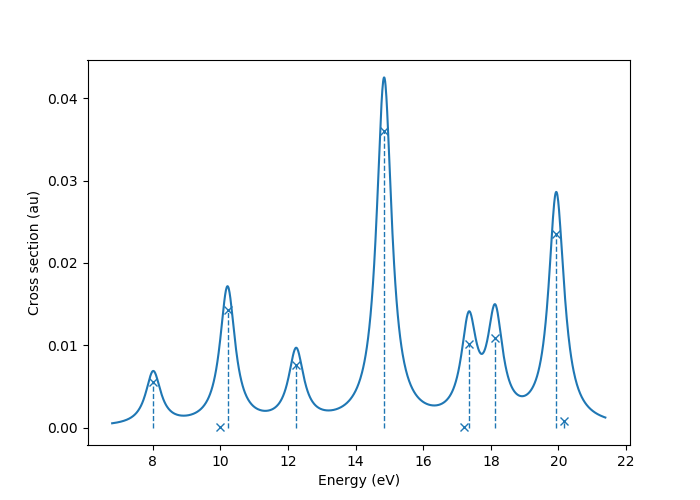
In this image crosses represent the actual computed value
for the absorption cross section for the obtained excited states.
To form the actual spectrum (solid blue line) these discrete
peaks are artificially broadened with an empirical broadening parameter.
Notice, that the adcc.ExcitedStates.plot_spectrum()
function does only prepare the spectrum inside Matplotlib,
such that plt.show() needs to be called in order to actuall see the plot.
This allows to simulaneously plot the spectrum from multiple
calculations in one figure if desired.
The adcc.ExcitedStates.plot_spectrum() function takes a number
of parameters to alter the default plotting behaviour:
Broadening parameters: The default broadening can be completely disabled using the parameter
broadening=None. If instead of useng lorentzian broadening, Gaussian broadening is preferred, selectbroadening="gaussian". The width of the broadening is controlled by thewidthparameter. Its default value is 0.01 atomic units or roughly 0.272 eV. E.g. to broaden with a Gaussian of width 0.1 au, callstate.plot_spectrum(broadening="gaussian", width=0.1)
Energy units: By default the energy on the x-Axis is given in electron volts. Pass the parameter
xaxis="au"to plot the energy in atomic units or passxaxis="nm"to plot the wave length in nanometers, e.g.state.plot_spectrum(xaxis="nm")
Intensity unit: By default the spectrum computes the absorption cross-section and uses this quantity for identifying the intensity of a particular transition. Other options include the oscillator strength by passing
yaxis="osc_strength".matplotlib options: Most keyword arguments of the Matplotlib
plotfunction are supported by passing them through. This includescoloror the used line marker. See the Matplotlib documentation for details.
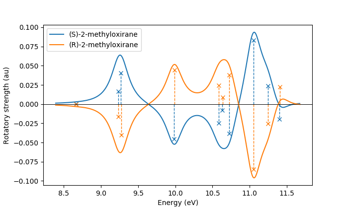
In the same manner, one can model the ECD spectrum of chiral molecules
with the adcc.ExcitedStates.plot_spectrum() function. An example
script for obtaining the ECD spectrum of (R)- and (S)-2-methyloxirane with ADC(2) can be
found in the examples folder.
The only difference to plotting a UV/Vis spectrum as shown above is to specify
a different yaxis parameter, i.e.
plots = state.plot_spectrum(yaxis="rotatory_strength")
which then, in the example, produces the following plot:
Reusing intermediate data
Since solving the ADC equations can be very costly various intermediates are only computed once and stored in memory. For performing a second ADC calculation for the identical system, it is thus wise to re-use this data as much as possible.
A very common use case is to compute singlets and triplets on top of a restricted reference. In order to achieve this with maximal data reuse, one can use the following pattern:
singlets = adcc.adc2(scfres, n_singlets=3)
triplets = adcc.adc2(singlets.matrix, n_triplets=5)
This will perform both an ADC(2) calculation for 3 singlets
as well as 5 triplets on top of the HF reference in scfres
by using the ADC(2) matrix stored in the singlets.matrix attribute
of the adcc.ExcitedStates class returned by the first
adcc.adc2() call, along with its its precomputed intermediates.
If the ADC method is to be varied between the first and the second run, one may at least reuse the Møller-Plesset ground state, like so
adc2_state = adcc.adc2(scfres, n_singlets=3)
adc2x_state = adcc.adc2x(adc2_state.ground_state, n_singlets=3)
which computes 3 singlets both at ADC(2) and ADC(2)-x level
again re-using information in the adcc.ExcitedStates class
returned by the first ADC calculation.
A slightly improved convergence of the second ADC(2)-x calculation
can be achieved, if we exploit the similarity of ADC(2) and ADC(2)-x
and use the eigenvectors from ADC(2) as the guess vectors for ADC(2)-x.
This can be achieved using the guesses parameter:
adc2_state = adcc.adc2(scfres, n_singlets=3)
adc2x_state = adcc.adc2x(adc2_state.ground_state, n_singlets=3,
                         guesses=adc2_state.excitation_vector)
This trick of course can also be used to tighten a previous ADC result in case a smaller convergence tolerance is needed, e.g.
# Only do a crude solve first
state = adcc.adc2(scfres, n_singlets=3, conv_tol=1e-3)

# Inspect state and get some idea what's going on
# ...

# Now converge tighter, using the previous result
state = adcc.adc2(state.matrix, n_singlets=3, conv_tol=1e-7,
                  guesses=state.excitation_vector)
Programmatic access to computed data
Note
This section should be written. Idea: Describe how to get data in a nice way.
Spin-flip calculations
Note
Describe: What is spin-flip? Why?
Two things need to be changed in order to run a spin-flip calculation with adcc.
Firstly, a triplet Hartree-Fock reference should be employed
and secondly, instead of using the n_states or n_singlets parameter,
one uses the special parameter n_spin_flip instead to specify the number
of states to be computed. An example for using PySCF to
compute the spin-flip ADC(2)-x states of hydrogen fluoride near the
dissociation limit.
import adcc
from pyscf import gto, scf

# Run SCF in pyscf aiming for a triplet
mol = gto.M(
    atom='H 0 0 0;'
         'F 0 0 3.0',
    basis='6-31G',
    unit="Bohr",
    spin=2  # =2S, ergo triplet
)
scfres = scf.UHF(mol)
scfres.conv_tol = 1e-13
scfres.kernel()

# Run ADC(2)-x with spin-flip
states = adcc.adc2x(scfres, n_spin_flip=5)
print(states.describe())
Since the first excited state in the case of spin-flip computations corresponds
to the singlet ground state, one requires an additional step to plot the excitation
spectrum. This can be conveniently achieved using the adcc.State2States class
which exposes results for transitions between excited states. In our case, we want to
plot the spectrum for transitions from the first excited state to all other higher-lying states:
s2s = adcc.State2States(states, initial=0)
s2s.plot_spectrum()
Another use case for adcc.State2States class for canonical ADC calculations
is the investigation of excited state absorption.
Core-valence-separated calculations
Note
Describe: What is CVS? Why?
For performing core-valence separated calculations,
adcc adds the prefix cvs_ to the method functions discussed already above.
In other words, running a CVS-ADC(2)-x calculation can be achieved
using adcc.cvs_adc2x(), a CVS-ADC(1) calculation
using adcc.cvs_adc1().
Such a calculation requires one additional parameter,
namely core_orbitals, which determines the number of spatial orbitals
to put into the core space. This is to say, that core_orbitals=1 will
not just place one orbital into the core space,
much rather one alpha and one beta orbital. Similarly core_orbitals=2
places two alphas and two betas into the core space and so on.
By default the lowest-energy occupied orbitals are selected to be part of
the core space.
For example, in order to perform a CVS-ADC(2) calculation of water, which places the oxygen 1s core electrons into the core space, we need to run the code (now using Psi4)
import psi4

# Run SCF in Psi4
mol = psi4.geometry("""
    O 0 0 0
    H 0 0 1.795239827225189
    H 1.693194615993441 0 -0.599043184453037
    symmetry c1
    units au
""")
psi4.core.be_quiet()
psi4.set_options({'basis': "cc-pvtz", 'e_convergence': 1e-13, 'd_convergence': 1e-7})
scf_e, wfn = psi4.energy('SCF', return_wfn=True)

# Run CVS-ADC(2) solving for 4 singlet excitations of the oxygen 1s
states = adcc.cvs_adc2(wfn, n_singlets=4, core_orbitals=1)
Restricting active orbitals: Frozen core and frozen virtuals
In most cases the occupied orbitals in the core region of an atom are hardly involved in the valence to valence electronic transitions. Similarly the high-enery unoccupied molecular orbitals typically are discretised continuum states or other discretisation artifacts and thus are rarely important for properly describing valence-region electronic spectra. One technique common to all Post-HF excited-states methods is thus to ignore such orbitals in the Post-HF treatment to lower the computational burden. This is commonly referred to as frozen core or frozen virtual (or restricted virtual) approximation. Albeit clearly an approximative treatment, these techniques are simple to apply and the loss of accuracy is usually small, unless core-like, continuum-like or Rydberg-like excitations are to be modelled.
In adcc the frozen core and frozen virtual approximations
are disabled by default. They can be enabled
in conjunction with any of The adcc.adcN family of methods via
two optional parameters, namely frozen_virtual
and frozen_core. Similar to core_orbitals,
these arguments allow to specify the number of spatial orbitals
to be placed in the respective spaces, thus
the number of alpha and beta orbitals to deactivate in the ADC treatment.
By default the lowest-energy occupied orbitals are selected
with frozen_core to make up the frozen core space and the
highest-energy virtual orbitals are selected with
frozen_virtual to give the frozen virtual space.
For example the code
import psi4

# Run SCF in Psi4
mol = psi4.geometry("""
    O 0 0 0
    H 0 0 1.795239827225189
    H 1.693194615993441 0 -0.599043184453037
    symmetry c1
    units au
""")
psi4.core.be_quiet()
psi4.set_options({'basis': "cc-pvtz", 'e_convergence': 1e-13, 'd_convergence': 1e-7})
scf_e, wfn = psi4.energy('SCF', return_wfn=True)

# Run FC-ADC(2) for 4 singlets with the O 1s in the frozen core space
states_fc = adcc.adc2(wfn, n_singlets=4, frozen_core=1)

# Run FV-ADC(2) for 4 singlets with 5 highest-energy orbitals
# in the frozen virtual space
states_fv = adcc.adc2(wfn, n_singlets=4, frozen_virtual=5)
runs two ADC(2) calulationos for 4 singlets. In the first the oxygen 1s is flagged as inactive by placing it into the frozen core space. In the second the 5 highest-energy virtual orbitials are frozen (deactivated) instead.
Frozen-core and frozen-virtual methods may be combined with
CVS calulations. When specifying both frozen_core
and core_orbitals keep in mind that the frozen core orbitals
are determined first, followed by the core-occupied orbitals.
In this way one may deactivate part of lower-energy occupied orbitals
and target a core excitation from a higher-energy core orbital.
For example to target the 2s core excitations of hydrogen sulfide one may run:
from pyscf import gto, scf
import adcc

mol = gto.M(
    atom='S  -0.38539679062   0 -0.27282082253;'
         'H  -0.0074283962687 0  2.2149138578;'
         'H   2.0860198029    0 -0.74589639249',
    basis='cc-pvtz',
    unit="Bohr"
)
scfres = scf.RHF(mol)
scfres.conv_tol = 1e-13
scfres.kernel()

# Run an FC-CVS-ADC(3) calculation: 1s frozen, 2s core-occupied
states = adcc.cvs_adc3(scfres, core_orbitals=1, frozen_core=1, n_singlets=3)
print(states.describe())
which places the sulfur 1s orbitals into the frozen core space and the sulfur 2s orbitals into the core-occupied space. This yields a FC-CVS-ADC(2)-x treatment of this class of excitations. Notice that this is just an example. A much more accurate treatment of these excitations at full CVS-ADC(2)-x level can be achieved as well, namely by running
states = adcc.cvs_adc3(scfres, core_orbitals=2, n_singlets=3)
Notice, that any other combination of CVS, FC and FV is possible as well. In fact all three may be combined jointly with any available ADC method, if desired.
Further examples and details
Some further examples can be found in the examples folder
of the adcc code repository.
For more details about the calculation parameters,
see the reference for The adcc.adcN family of methods.