Theoretical review of ADC methods
The polarisation propagator  is a quantity from many-body
perturbation theory [Fet71].
Its relationship to electronically excited states spectra can be understood
from the fact
that its poles are located exactly at the vertical excitation energies
is a quantity from many-body
perturbation theory [Fet71].
Its relationship to electronically excited states spectra can be understood
from the fact
that its poles are located exactly at the vertical excitation energies
 [Fet71][Sch82].
Here,
[Fet71][Sch82].
Here,  is the energy of the ground state of the
exact
is the energy of the ground state of the
exact  -electron Hamiltonian
  ,
and
,
and  is the energy corresponding to excited state
 .
The structure of close to these poles
depends both on the ground state
.
The structure of close to these poles
depends both on the ground state  and excited state
,
such that, e.g., transition properties [Sch82][Sch18]
may be extracted from as well.
and excited state
,
such that, e.g., transition properties [Sch82][Sch18]
may be extracted from as well.
Taking this as a starting point,
the algebraic-diagrammatic construction scheme
for the polarisation propagator (ADC)
examines an alternative representation of the
polarisation propagator [Sch82],
the so-called intermediate-state representation (ISR).
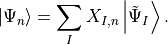
In this formalism, a set of creation and annihilation operators is
applied to the exact ground state
and the resulting precursor states are orthogonalised block-wise according
to excitation class [Sch91].
This procedure yields the so-called intermediate states
 ,
which are then employed to represent the polarisation propagator.
A careful inspection of the resulting expression for
and its poles allows to relate the
intermediate states (IS) to the excited states
of the Hamiltonian [Sch91]
by a unitary transformation
,
which are then employed to represent the polarisation propagator.
A careful inspection of the resulting expression for
and its poles allows to relate the
intermediate states (IS) to the excited states
of the Hamiltonian [Sch91]
by a unitary transformation
The expansion coefficients  satisfy a Hermitian eigenvalue problem [Sch91]
(1)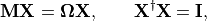
where  is the diagonal matrix of excitation energies and
 is the so-called ADC matrix.
Its elements are directly accessible by representing the shifted Hamiltonian using IS, namely
is the so-called ADC matrix.
Its elements are directly accessible by representing the shifted Hamiltonian using IS, namely
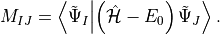
From the ADC eigenvectors in the IS basis,
one may compute the density matrix  for an excited state
  or the transition density matrices
 between state
  and ,
in the molecular orbital (MO) basis [ST04][WRH+14].
Contracting these densities with the MO representation
and ,
in the molecular orbital (MO) basis [ST04][WRH+14].
Contracting these densities with the MO representation  of a one-particle operator
  allow to compute arbitrary
state properties
allow to compute arbitrary
state properties  or transition properties
  through
In this way, e.g., the MO representation of the dipole operator
may be contracted with to
obtain the transition dipole moment between
states and and from this the oscillator strength.
Linear and non-linear molecular response properties,
e.g., static polarizabilities or two-photon absorption cross-sections,
are also accessible via this framework
[TKWS06][KRW+12][FRDN17].
As described so far, the above formalism builds the IS basis on top of
the exact -electron ground state and is thus exact as well.
For practical calculations, however,
the ADC scheme is not applied to the exact ground state,
but to a Møller-Plesset ground state at order
of perturbation theory.
The resulting ADC method is named ADC()
and is by construction consistent
with an MP() ground state.
Detailed derivations and the resulting expressions for the ADC matrix
as well as the aforementioned
densities and
for various orders can be found in the
literature [Sch82][Sch91][WRH+14][DW14][Sch18]
and will not be discussed here.
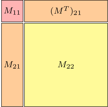
Fig 1a. Schematic ADC matrix¶ |
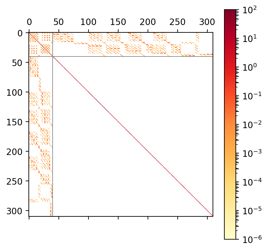
Fig 1b. ADC(2) matrix of STO-3G water¶ |
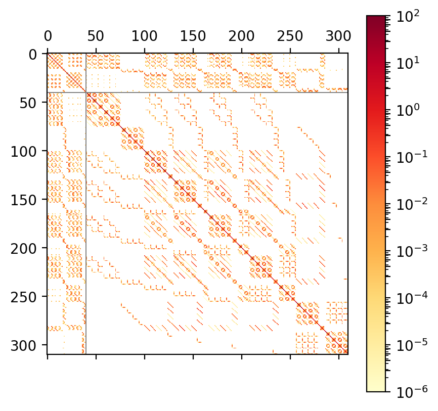
Fig 1c. ADC(3) matrix of STO-3G water¶ |
As a result of the construction of ADC() as excitations on top of
an MP() ground state, the matrix
exhibits a block structure, shown in Figure 1a.
In this the singles block is denoted  ,
the doubles block
,
the doubles block  and the
coupling block
and the
coupling block  .
One may construct perturbation expansions for the individual blocks as well.
For example in ADC(2) the lower-right block
is only present in zeroth order.
In ADC(3) on the other hand this block is present at first order,
which makes it consistent with an MP(3) ground state.
In contrast, ADC(2)-x is an emph{ad hoc} modification of ADC(2),
where only the doubles-doubles block is treated first order like in ADC(3),
but the remaining blocks remain at the same order as in ADC(2) [DW14].
.
One may construct perturbation expansions for the individual blocks as well.
For example in ADC(2) the lower-right block
is only present in zeroth order.
In ADC(3) on the other hand this block is present at first order,
which makes it consistent with an MP(3) ground state.
In contrast, ADC(2)-x is an emph{ad hoc} modification of ADC(2),
where only the doubles-doubles block is treated first order like in ADC(3),
but the remaining blocks remain at the same order as in ADC(2) [DW14].
On top of this block structure the individual blocks are sparse
as well, see Figure 1b and c.
This sparsity is a direct consequence of the selection rules obtained from
spin and permutational symmetry in the tensor contractions required
for computing .
To exploit this sparsity when diagonalising
the matrix (1),
adcc follows the conventional approach [DW14][WRH+14]
to use contraction-based, iterative
eigensolvers, such as the Jacobi-Davidson [Dav75].
Furthermore, all tensor operations in the required ADC matrix-vector products
are performed on block-sparse tensors.
For an optimal performance the spin and permutational symmetry of the ADC equations
need to be taken into account when setting up the block tiling
along the tensor axes.
In this setting the computational scaling of ADC(2) is given as  where is the number of orbitals,
whereas ADC(2)-x and ADC(3) scale as
where is the number of orbitals,
whereas ADC(2)-x and ADC(3) scale as  .
This procedure additionally ensures the numerical stability of the eigensolver
with respect to the excitation manifold.
That is to say, that (for restricted references) spin-pure guess vectors
always lead to eigenvectors from the same manifold,
such that the excitation manifold to probe can be reliably selected
via the guesses without employing a spin-adapted basis. [DW14]
.
This procedure additionally ensures the numerical stability of the eigensolver
with respect to the excitation manifold.
That is to say, that (for restricted references) spin-pure guess vectors
always lead to eigenvectors from the same manifold,
such that the excitation manifold to probe can be reliably selected
via the guesses without employing a spin-adapted basis. [DW14]
One important modifications of the ADC scheme as discussed above is the core-valence separation (CVS) [CDS80][TMG+00][WWD14b][WWD14a][WHWD15]. In this approximate ADC treatment targeting core-excited states, the strong localisation of the core electrons and the weak coupling between core-excited and valence-excited states is exploited to decouple and discard the valence excitations from the ADC matrix. This lowers the number of the actively treated orbitals and thus the computational demand for solving the ADC eigenproblem (1). The validity of this approximation has been analysed in the literature and is backed up by computational studies comparing with experiment [ND18][FD19]. With this, ADC can be used for considering core-excited states, and subsequent studies have also established the ability of calculating non-resonant X-ray emission spectra [FD19] and resonant inelastic X-ray scattering [RDN17]. Other variants of ADC include spin-flip [LWD15], where a modified Davidson guess allows to treat processes of simultaneous excitation and spin-flip, tackling few-reference problems in an elegant and consistent way [LRD16][LTMartinezD17]. Similar to other CI-like methods the range of orbitals which are considered for building the intermediate states may also be artificially truncated. For example, when considering valence-excitations, excitations from the core orbitals may be dropped leading to a frozen-core (FC) approximation. Similarly, high-energy virtual orbitals may be left unpopulated, leading to a frozen-virtual (FV) or restricted-virtual approximation [YD17].